This article explains What Is Transfer Learning in AI? And how it works, and when it makes sense to start with a pre-trained model. It also covers the difference between feature extraction and fine-tuning, with a practical example in Python.
Have you ever wondered how an AI model can learn to spot product defects when you have only a few hundred examples of damaged parts?
Imagine you run a factory that makes plastic housings. Your inspection camera captures thousands of photos of acceptable parts, but your team has only a small collection of confirmed cracks, chips, and dents. You want the model to flag damaged parts for review while keeping the number of false alerts manageable.
This is one practical use of transfer learning. You can start with an image model that has already learned to recognise patterns such as edges, shapes, and textures. You then use labelled photos from your production line to train a new classifier that distinguishes acceptable parts from defective ones.
The model’s earlier training gives you a starting point. Your team still needs to define which marks count as defects and test the model on production batches it has never seen. A model can achieve high overall accuracy when defects are rare, so count how many defects it misses and how many acceptable parts it flags.
Whether you are building your first image classifier, routing customer support tickets, or adapting a speech recognition model for regional accents, understanding transfer learning can help you decide which model to start with, what examples to collect, and how to judge the result.
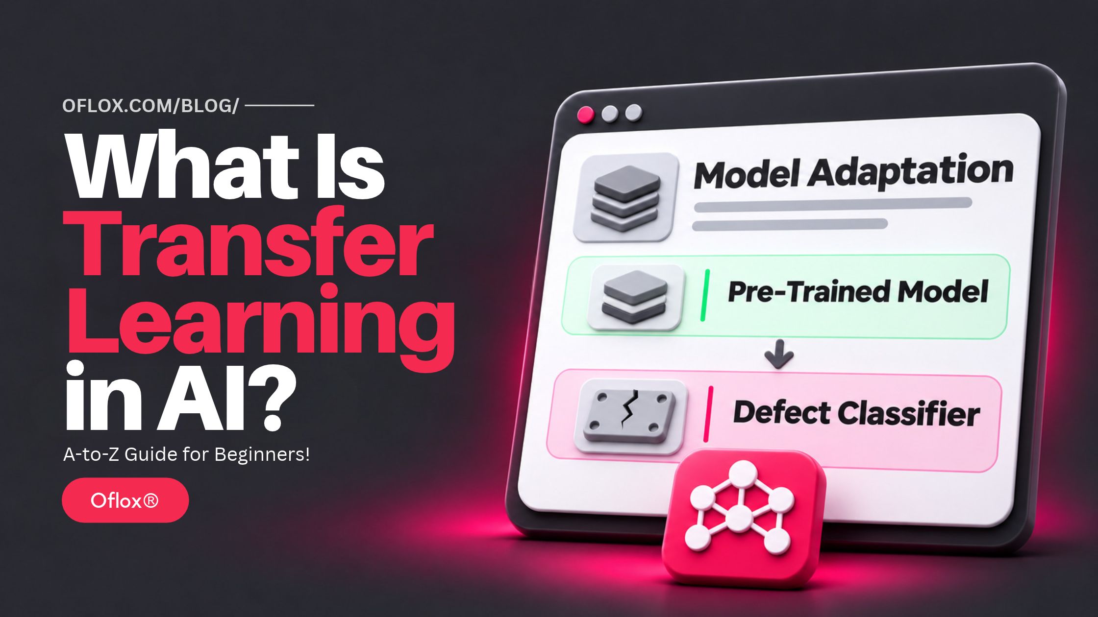
In this Oflox® guide, we will walk through a product inspection example, compare feature extraction with fine-tuning, and show you how to adapt a pre-trained ResNet18 model using Python and PyTorch.
Let’s explore it together!
Table of Contents
What Is Transfer Learning in AI?
Transfer learning in AI is a technique that uses knowledge learned from one task or dataset to help a model perform a different but related task. For example, an image model trained on general photographs can be adapted to classify photos of factory products as acceptable or defective.
Think of a quality inspector joining a new factory. The inspector already knows how to examine surfaces, spot irregularities, and compare finished parts. The new employer teaches them which scratches are acceptable, which cracks require rejection, and where the most common defects appear. The inspector’s existing skills make that training easier.
In AI, the skills being reused often come from the model’s weights. Weights are numerical values the model learns during training. In an image model, they help convert pixels into useful features, such as edges, textures, and shapes. A new classifier can use those features to make decisions about your products.
Here’s what the common transfer learning terms mean in practice:
| Term | Simple meaning | Product inspection example |
|---|---|---|
| Pre-trained model | A model that has already completed an earlier training stage | An image model trained on ImageNet |
| Source domain | The type of data used in the original training | General photographs |
| Source task | What the model originally learned to do | Recognise categories in those photographs |
| Target domain | The type of data the adapted model will handle | Images from your factory camera |
| Target task | What you want the adapted model to do | Classify a part as acceptable or defective |
| Backbone | The part of the model that extracts features | The layers of ResNet18 that process each image |
| Classification head | The part that turns features into class scores | A new layer that scores the two inspection categories |
Transfer can happen when the task changes, when the data changes, or when both change. For example, moving an existing defect classifier from one production line to another can keep the same labels while introducing different lighting and camera angles.
Why Is Transfer Learning Important?
Collecting data and labelling it are two different jobs. A company may have years of support conversations but only a small number tagged correctly by issue type. A factory may capture thousands of images every day, while defects appear infrequently and take time for inspectors to confirm.
Transfer learning gives these teams a way to run a useful experiment with the labelled examples they already have. They can test whether a pre-trained model’s features help, study the mistakes, and decide which data would make the next experiment more informative.
For instance, imagine that the factory model detects dents reliably but misses hairline cracks. The team reviews those photos and finds that the cracks are barely visible after the images are resized. Closer camera framing could improve the result more than another round of training. If the cracks are clearly visible and the model still misses them, the team might collect more examples across different product finishes and compare a fine-tuned model.
There is also a difference between training cost and deployment cost. Updating a small classification layer can make adaptation cheaper. The full backbone still processes each new image, so an inexpensive model to train may take too long to make a prediction on a factory computer. Measure both costs when choosing a model for a business workflow.
A Brief History of Transfer Learning
Here’s how transfer learning evolved from early research on reusing knowledge to today’s pre-trained models that can be adapted for new tasks.
1. What Is Transfer Learning in AI
In their 2010 survey, Sinno Jialin Pan and Qiang Yang reviewed transfer learning research around three questions. What can be transferred? How should it be transferred? When will it help?
The field covers more than reusing neural network weights. Depending on the problem, researchers can transfer information from examples, feature representations, or model parameters. Downloading a pre-trained checkpoint and adapting it is the approach you are most likely to encounter in a practical deep learning tutorial.
2. Deep learning made visual features easier to reuse
In 2014, Jason Yosinski and colleagues studied which features in deep neural networks could transfer between image classification tasks. They found that transfer generally became harder as the original and new tasks grew more different.
That distinction matters when you choose a starting model. An image model trained on ordinary photographs might be a reasonable baseline for an RGB camera on a production line. For thermal imagery, you have a reason to test a model trained on data that more closely resembles what your camera captures.
3. Larger models made smaller updates more attractive
As language models grew, updating every weight for each application became more demanding. In 2021, the LoRA paper introduced a method that keeps the original weights frozen while learning much smaller updates. Later vision research, such as DINOv3, showed how a single self-supervised backbone could produce features for several downstream tasks. Together, these approaches give teams more options for deciding what to reuse and what to train.
How Does Transfer Learning Work?
Here’s how to apply transfer learning to a factory inspection project, from defining the problem to measuring the result.
1. Decide what the model should predict
Start with a decision the model can make from the information it receives. In this example, it looks at one photo and flags potentially defective parts for an inspector to review.
Write down what counts as a defect. Should a shallow cosmetic scratch be accepted? Does a chip near a screw hole require rejection? What should an inspector do if glare hides part of the surface? Include example photos in your labelling guide so different people apply the same rules.
2. Select a suitable pre-trained model
For standard colour photos, an ImageNet-pre-trained ResNet18 is a practical starting point. Check the expected input size, how the model normalises colours, and whether its weights can be used under the terms of your project.
Look at your photos before making a decision. If the smallest defect is only a few pixels across, resizing the image for a standard model may make the defect harder to see. In that situation, try closer camera framing or crop to the inspection area before settling on an input size.
3. Split the data into training, validation, and test sets
The training set teaches the classifier. The validation set helps you choose a model and decide how sensitive it should be. The test set measures performance after those choices are settled.
Keep related images in the same split. If you have five photos of one part, putting three in training and two in testing can make performance look better than it will be on new parts. Split by physical item, production batch, or date based on what you want to measure. Holding out a later batch is useful when your main question is how the model will handle future production.
4. Replace the original classification layer
The original ResNet18 classification layer scores ImageNet categories. Your factory needs two scores, one for acceptable and one for defective. Replace the original layer with a new one that matches those labels.
Then freeze the backbone and train the new classifier. Freezing prevents the optimiser from updating the backbone’s weights. This first experiment tells you whether the existing image features are useful for your task.
5. Measure the errors that matter
Suppose you have 1,000 validation images and 20 show defects. A model that calls every part acceptable would achieve 98% accuracy while catching zero defects. That accuracy figure tells you very little about whether the model can help the inspection team.
Now imagine a model flags 30 parts. Sixteen are defective and 14 are acceptable. Its recall for defects is 80% because it catches 16 out of 20 defects. Its precision for defects is about 53% because 16 out of 30 flagged parts are genuinely defective.
Those two figures help the team decide whether the model fits the workflow. The team can see how many defects slip through and how many acceptable parts inspectors have to review. Choose the alert threshold on the validation set and confirm the resulting performance on the independent test set.
6. Fine-tune if the baseline leaves a meaningful gap
Try unfreezing the last block of the backbone if the fixed features work reasonably well and the remaining errors suggest the model could learn more from your images. Train the unfrozen layers with a lower learning rate and compare the result on the same validation batches.
Review the images behind the errors too. Fine-tuning may help if the model struggles with a distinctive texture it can see in the input. If a centre crop removes a crack entirely, the image pipeline needs attention first.
Feature Extraction vs Fine-Tuning
Feature extraction keeps the pre-trained backbone fixed and trains a new model on its outputs. Fine-tuning adapts some or all of the pre-trained network, or adds small trainable updates to it. Both are ways to apply transfer learning.
| Approach | What gets trained? | When to try it |
|---|---|---|
| Fixed feature extraction | A new classifier on top of the frozen backbone | You want a quick baseline with limited labelled data |
| Partial fine-tuning | The new head and selected pre-trained layers | The existing features help, but some errors suggest the model needs more adaptation |
| Full fine-tuning | All model parameters can be updated | You have enough relevant data and compute to compare broader adaptation |
| Parameter-efficient fine-tuning | A small set of added or selected parameters, depending on the method | You are adapting a large model or maintaining several variants |
LoRA, short for Low-Rank Adaptation, is an example of parameter-efficient fine-tuning. A software team could use the same base language model and train separate updates for tasks like routing support tickets and extracting fields from documents. Each adaptation still needs its own evaluation because it changes a different part of the workflow.
Transfer Learning vs Training From Scratch
Training from scratch typically starts with randomly initialised weights. Transfer learning starts with knowledge already learned from another task or dataset. The best choice depends on your data, the available checkpoints, and the hardware that will run the model.
| Factor | Transfer learning | Training from scratch |
|---|---|---|
| Starting point | Existing model weights or features | Randomly initialised model weights |
| Labelled target data | Can be effective with fewer examples when the features transfer well | Often needs more examples for the model to learn useful features |
| Training effort | Can be lower when most weights are frozen | Depends on the architecture and training schedule |
| Deployment constraints | Largely shaped by the chosen backbone | Can be designed around the intended hardware |
| Main challenge | Finding a checkpoint that fits your data and task | Learning reliable features from the data you can collect |
Suppose the inspection camera only needs to check whether a bright sticker appears inside a marked rectangle. A basic image-processing rule could be a sensible starting point. For cracks that vary in shape, size, and position, a pre-trained image model is worth evaluating. Compare each approach on fresh production images, including the cases that cause the most expensive errors.
Transfer Learning Example Using Python and PyTorch
Here’s how to use a pre-trained ResNet18 to classify images as acceptable or defective. The example trains the new classification head, selects it using validation loss, and reports how well it detects defects on the test set.
Install compatible versions of torch and torchvision before running the script. The first run downloads the pre-trained weights if they are unavailable locally.
1. Organise your images
Place the following folders in the directory where you will run the script. Make sure every split contains both classes. Assign entire parts or batches to a split before copying the photos.
product_photos/
  train/
    acceptable/
    defective/
  val/
    acceptable/
    defective/
  test/
    acceptable/
    defective/
This example uses the preprocessing supplied with the model weights. It resizes, centre-crops, and normalises the photos. Check a few processed images first, particularly when parts or defects appear near the edge of the frame.
2. Train and evaluate the classifier
from copy import deepcopy
from pathlib import Path

import torch
from torch import nn
from torch.utils.data import DataLoader
from torchvision.datasets import ImageFolder
from torchvision.models import ResNet18_Weights, resnet18

torch.manual_seed(42)
device = torch.device("cuda" if torch.cuda.is_available() else "cpu")
root = Path("product_photos")

weights = ResNet18_Weights.DEFAULT
preprocess = weights.transforms()
expected_classes = {"acceptable", "defective"}

datasets = {}
loaders = {}

for split in ("train", "val", "test"):
    dataset = ImageFolder(root / split, transform=preprocess)
    if set(dataset.classes) != expected_classes:
        raise ValueError(f"{split} must contain acceptable and defective images.")

    datasets[split] = dataset
    loaders[split] = DataLoader(
        dataset, batch_size=16, shuffle=(split == "train")
    )

model = resnet18(weights=weights)
model.requires_grad_(False)
model.fc = nn.Linear(model.fc.in_features, len(expected_classes))
model.to(device)

loss_fn = nn.CrossEntropyLoss()
optimizer = torch.optim.AdamW(model.fc.parameters(), lr=1e-3)
best_loss = float("inf")
best_head = None

for epoch in range(5):
    # Keep the frozen backbone's batch normalisation statistics fixed.
    model.eval()
    model.fc.train()

    for images, labels in loaders["train"]:
        images, labels = images.to(device), labels.to(device)
        optimizer.zero_grad()
        loss = loss_fn(model(images), labels)
        loss.backward()
        optimizer.step()

    model.eval()
    total_val_loss = 0.0
    with torch.inference_mode():
        for images, labels in loaders["val"]:
            images, labels = images.to(device), labels.to(device)
            batch_loss = loss_fn(model(images), labels)
            total_val_loss += batch_loss.item() * labels.size(0)

    val_loss = total_val_loss / len(datasets["val"])
    print(f"Epoch {epoch + 1}: validation loss {val_loss:.4f}")

    if val_loss < best_loss:
        best_loss = val_loss
        best_head = deepcopy(model.fc.state_dict())

if best_head is None:
    raise RuntimeError("Training produced no usable validation checkpoint.")

model.fc.load_state_dict(best_head)
model.eval()

defect_id = datasets["test"].class_to_idx["defective"]
true_positives = false_positives = false_negatives = 0

with torch.inference_mode():
    for images, labels in loaders["test"]:
        predictions = model(images.to(device)).argmax(dim=1).cpu()
        flagged = predictions == defect_id
        defective = labels == defect_id

        true_positives += (flagged & defective).sum().item()
        false_positives += (flagged & ~defective).sum().item()
        false_negatives += (~flagged & defective).sum().item()

flagged_count = true_positives + false_positives
actual_defects = true_positives + false_negatives

if flagged_count:
    print(f"Defect precision: {true_positives / flagged_count:.1%}")
else:
    print("Defect precision: undefined because no photos were flagged.")

if actual_defects:
    print(f"Defect recall: {true_positives / actual_defects:.1%}")
else:
    print("Defect recall: undefined because the test set has no defects.")

print(f"Missed defects: {false_negatives}")
3. Understand what the numbers tell you
The script uses the class with the higher score as its initial decision. For a real inspection workflow, you might want to flag a part at a lower defect score so an inspector can catch more questionable items. Test potential thresholds on the validation set and compare how many extra reviews each option creates.
Also pay attention to the number of defective examples behind the percentage. If your test set has only five defective photos, missing one drops recall by 20 percentage points. Report counts alongside percentages and review examples across different batches and defect types before drawing conclusions. The code is an illustrative walkthrough. Its performance depends on the dataset you supply.
Real-World Applications of Transfer Learning
Here’s how the same approach can help with different kinds of AI projects:
| Application | What can be reused? | What should you test? |
|---|---|---|
| Product inspection | A pre-trained image model | Detection of cracks, dents, and chips across batches and finishes |
| Customer support routing | A pre-trained language model or encoder | Correct assignment of fresh tickets, including rare categories |
| Speech recognition | A pre-trained audio model | Transcription quality across accents, noise levels, and technical terms |
| Invoice processing | A model that represents text and page layout | Accuracy of individual fields across vendors and templates |
| Image search | A pre-trained vision model that produces embeddings | Whether visually relevant items appear near the top of the results |
Consider a customer message that says, “Payment ho gaya but invoice nahi mila.” A general language model might understand the message. The support team still needs to decide whether that issue should go to billing, payment support, or the team responsible for invoices. Past tickets labelled according to the company’s rules can teach a classifier how to route similar requests.
Invoice processing has a different challenge. A model may correctly extract invoice numbers from familiar layouts but pick up a purchase order number on a new supplier’s template. If you want to know how it will handle new vendors, reserve complete vendor templates for testing and check each extracted field separately.
Key Features and Benefits of Transfer Learning
Here’s what makes transfer learning practical for developers and businesses:
- Reusable features. An existing model may already capture patterns relevant to your data, such as edges in images or relationships between words in text.
- Flexible adaptation. You can train a small classifier first, unfreeze selected layers later, or use parameter-efficient updates for a larger model.
- A faster first experiment. A frozen model and a small head give you an early indication of whether your labels and inputs are sufficient to make progress.
- Lower adaptation costs in suitable projects. Updating fewer parameters can reduce memory and compute requirements during training.
- Reuse across related tasks. One vision backbone can support several classifiers, while each classifier keeps its own class definitions and acceptance criteria.
Limitations and Common Challenges
Transfer learning depends on how well the original model fits your problem. Here are the issues to check before relying on an adapted model:
| Challenge | What it looks like | How to investigate it |
|---|---|---|
| Negative transfer | The adapted model performs worse than a relevant baseline | Compare both on the same held-out split and metric |
| Domain mismatch | Results drop after a change in lighting, language, device, or input format | Report performance separately for each relevant condition |
| Inherited weaknesses | The model makes more errors on inputs underrepresented in its training | Include those cases in the evaluation and inspect errors directly |
| Overfitting | Training improves while performance on new batches drops | Compare the frozen baseline with partial fine-tuning |
| Preprocessing errors | Important details disappear during cropping, resizing, or augmentation | Inspect the images the model actually receives |
| Deployment constraints | The model works in a notebook but runs too slowly on the target device | Measure end-to-end prediction time on the intended hardware |
A drop in results can also come from inconsistent labels. If two inspectors disagree about whether a certain scratch requires rejection, review the labelling rule before changing the model. The model should learn a decision that the team can apply consistently.
5+ Helpful Tools for Transfer Learning
Here’s where to start based on the type of model you want to build:
| Tool | What you can use it for |
|---|---|
| PyTorch and TorchVision | Load pre-trained image models, reuse their transforms, and write a custom training loop |
| TensorFlow and Keras | Build an image classification prototype within a Keras workflow |
| Hugging Face Transformers and PEFT | Work with supported pre-trained models and experiment with efficient fine-tuning |
| scikit-learn | Train a simple classifier on exported features and compare classification metrics |
| MLflow | Track model versions, experiment settings, and evaluation results |
| OpenVINO | Optimise and run adapted AI models on Intel hardware. |
For a first computer vision project, start with two runs on the same dataset split. Train a frozen backbone with a new head, then try partial fine-tuning if the baseline warrants it. Record the model version, class definitions, preprocessing, and defect counts so you can explain the difference between the runs.
Expert Tips and Common Mistakes
Here’s how to avoid common transfer learning mistakes, from mixing photos of the same product across data splits to fine-tuning before you understand why the model misses defects.
- Look at the actual mistakes before changing the model: Review missed defects with the inspection team. Check whether the images contain motion blur, glare, an unfamiliar finish, or damage that occupies only a small area. If errors come mostly from the late shift, investigate the lighting or camera settings before tuning model parameters.
- Compare results at a similar review volume: A model that flags twice as many products may find more defects and create more work for the team. For a fair comparison, check how many defects each model catches at a review volume the inspectors can manage. This makes the test relevant to the business decision.
- Check whether augmentation preserves the label: A horizontal flip is often harmless for a symmetrical part. The same flip can put an important notch on the wrong side of an asymmetric component. Blur can erase a hairline crack while leaving the image labelled defective. Open a sample of the transformed photos and confirm that an inspector can still make the intended decision.
- Test the workflow from input to alert: Capture a fresh photo on the production device. Run it through the deployed preprocessing steps and confirm that the correct class label appears in the review queue. An end-to-end test can reveal a different crop in production, reversed class labels, or a timeout between the camera and the inspection screen.
- Keep the test set independent: Use the validation set to choose training settings, thresholds, and model versions. If you repeatedly change the model after reading the same test results, that set starts influencing your decisions. An independent holdout gives you a better estimate of how the final choice will perform on genuinely new inputs.
FAQs:)
A. Transfer learning means taking a model that has already learned something useful and applying that learning to a new problem. For example, a model trained on general images can be adapted to recognise damage in product photos.
A. Transfer learning is the broader approach of reusing earlier learning. Fine-tuning is one method of applying it. Another is to keep the pre-trained model fixed and train a separate classifier on the features it produces.
A. The amount depends on the diversity of your inputs, the number of labels, and how closely the pre-trained model fits the new task. Start with a representative pilot and add examples where errors cluster. Keep enough separate data to evaluate those cases.
A. Yes. This is called negative transfer. It can happen when earlier learning is poorly suited to the target problem. Compare the transferred model with a relevant baseline on the same evaluation data.
A. Yes. A pre-trained language model can be adapted for tasks such as ticket classification, structured extraction, and generating replies in a specific format. Full fine-tuning and parameter-efficient methods such as LoRA are two options.
A. Yes. A small image model with a frozen backbone can be used for a CPU-based experiment, especially when the dataset is small. You can also compute the features once and train a lightweight classifier on them. Try a short run to see what the full workload will take on your hardware.
Conclusion:)
Understanding what transfer learning is in AI helps you decide whether a pre-trained model can solve a problem with the data you already have. Start with one clear decision, build a simple baseline, and judge the result on fresh examples that represent how the system will be used.
For product inspection, count the defects the model misses and the number of parts it sends for review. For customer support, check whether fresh messages reach the right team. These results tell you whether to improve the data, fine-tune the model, or choose a different approach.
At Oflox®, we approach custom software and AI development by defining what the system must decide, what data it can use, and how the client will judge the result. If you are planning an AI project, share a sample of your inputs and the workflow you want to improve.
“A pre-trained model earns its place when it helps you make better decisions on your own data.” — Suggested quote for Mr Rahman, Oflox®
Read also:)
- Difference Between JSON and XML With Example: A-to-Z Guide!
- How Website Forms Turn Visitors Into Potential Customers?
- What Is an LLM Gateway? A-to-Z Guide for Beginners!
Have you used transfer learning in an AI project? Share which pre-trained model you chose, what you adapted it for, and the biggest challenge you faced in the comments below.